The \(l_1\) regularized optimization problems are quite common in machine learning. They lead to a sparse solution to the modelling problem. Consider the following optimization problem with \(l_1\) penalty^[1].

\[ \min_{\theta \in \mathbb R} f(\theta) := h(\theta) + \lambda |\theta| \]

Where \(\theta\) are the parameters of the model \(f\) to be optimized. Let us study the reparameterization \(\theta = \mu \circ \nu\) for all \(\theta \in \mathbb R\), where \(\circ\) represents the element-wise (Hadamard) product of the vectors \(\mu\) and \(\nu\). This is called the Hadamard product parameterization (HPP) or simply the Hadamard paramterization^[2]. Then the equation (1) can be written as

\[ \begin{aligned} \min_{\theta \in \mathbb R} f(\theta) &= h(\theta) + \lambda |\theta| \\ % &\leq h(\theta) + \lambda \|\theta\|_2 \\ &=h(\mu \circ \nu) + \lambda \sum_i |\mu_i \nu_i| \\ &= h(\mu \circ \nu) + \lambda \sum_i \sqrt{\mu_i^2 \nu_i^2} \\ &\leq h(\mu \circ \nu) + \lambda \bigg ( \sum_i \frac{\mu_i^2 + \nu_i^2}{2} \bigg ) && {\color{OrangeRed}\text{AM-GM Inequality}}\\ &\leq h(\mu \circ \nu) + \frac{\lambda}{2} \big ( \| \mu\|_2^2 + \|\nu\|_2^2 \big ) \\ & \leq \min_{\mu, \nu \in \mathbb R} g(\mu, \nu) \end{aligned} \]

Therefore, the auxiliary optimization function is

\[ \min_{\mu, \nu \in \mathbb R} g(\mu, \nu) := h(\mu \circ \nu) + \frac{\lambda}{2} \big ( \| \mu\|_2^2 + \|\nu\|_2^2 \big ) \]

The above function is constructed rather purposefully to satisfy the following properties.

1. The over-parameterized function \(g(\mu, \nu)\) is an upper bound to our optimization function \(f(\theta)\), i.e. \(g(\mu,\nu) \geq f(\mu \circ \nu), \forall \mu,\nu \in \mathbb R\). The equality occurs where \(|\mu| = |\nu|\) as can be observed from equation (2).

2. The function \(g(\mu, \nu)\) satisfies the equality \(\inf f = \inf g\). This means that the optima (minima in this case) of \(f\) is equal to the optima of \(g\). In other words, if \(\mu\) and \(\nu\) are optimal (in terms of \(l_2\)), then \(\mu \circ \nu\) is an optimal (in terms of \(l_1\)) value of \(\theta\).

Moreover, since \(g(\mu, \nu)\) uses the \(l_2\) regularization, it is differentiable and biconvex. Thus, the auxiliary function is amenable to gradient-based optimization algorithms like SGD, Adam, etc. Interestingly, Ziyin et. al.^[3] also proved a stronger property compared to \(\inf f = \inf g\). They show that at all stationary points of (3), \(|\mu_i| = |\nu_i| \; \forall i \) and every local minima of \(g(\mu, \nu)\), given by equation (3) is a local minima of \(f(x)\), given by equation (1).

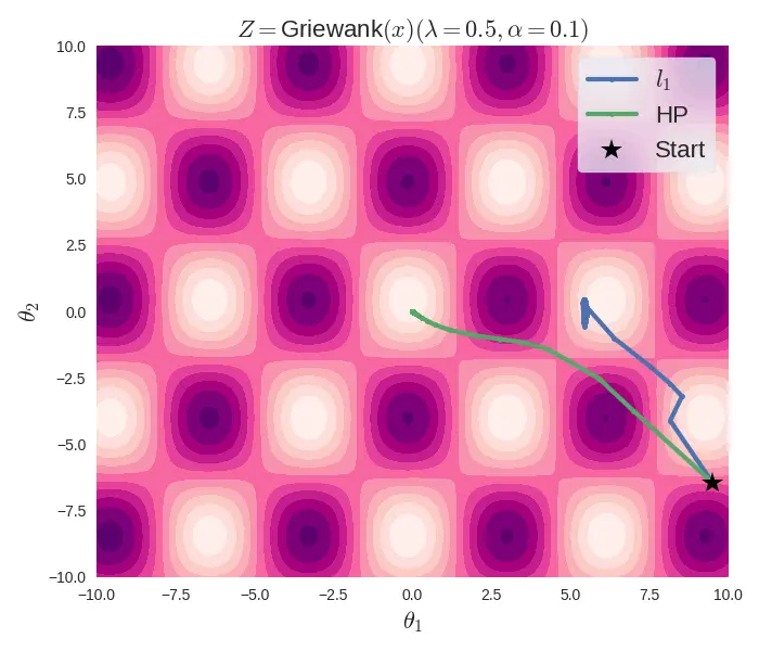
Optimization trajectory of l1 and HP regularizations

The above figure shows that, for the same initial conditions and optimization parameters, the \(l_1\) regularized objective function (Griewank, in this case) gets stuck in a local minima, while the Hadamard-parameterized function correctly reaches the global minima, which is at \((0, 0)\). Note that the \(l_1\) regularized objective can be used with Pytorch's SGD optimizer, as they use a subgradient of 1 at the non-differentiable point. But this is a convention, as the subgradient of \(|x|\) at \(0\) is the set \([-1, 1]\).

  Lastly, similar to interpreting the \(l_1\) and \(l_2\) regularizers in least-squares problems as Laplacian and Gaussian priors respectively, the equation (3) can also be examined through a probabilistic framework. Here, with the parameters \(\mu\) and \(\nu\) subject to \(l_2\) norm regularization, they can be construed as being governed by a Gaussian prior distribution \(\mathcal{N}(0, 2/\lambda)\). This implies a regularization effect on the components \(\mu\) and \(\nu\).

---

[1]	TIL, that the notation \(l_p\) is reserved for vectors while the uppercase notation \(L_p\) is for operators and functions. So, the appropriate notations are \(l_2(x)\) and \(L_2[\phi(x)]\) for vector \(x\) and the function \(\phi(x)\) respectively.

[2]	Hoff, P. D. (2017). Lasso, fractional norm and structured sparse estimation using a hadamard product parametrization. Comput. Stat. Data An., 115:186–198. ArXiv Link.

[3]	Ziyin, L. & Wang, Z. (2023). spred: Solving L1 Penalty with SGD. Proceedings of the 40th International Conference on Machine Learning, in Proceedings of Machine Learning Research 202:43407-43422 ArXiv Link