Let's say we have some data samples \(\mathcal D = \{\mathbf x | \mathbf x \in \mathbb R^{d}\}\) in \(d-\)dimensions. Defining a distance metric in to capture the relationship between two points \(\mathbf x_1\) and \(\mathbf x_2\) is an important problem. If we simply take the space \(\mathbb R^d\) to be Euclidean, we can then directly compute the Euclidean distance as

\[ d_E(\mathbf x_i, \mathbf x_j) = \|\mathbf x_i - \mathbf x_j\|_2 \qquad {\color{OrangeRed} \text{(Euclidean Distance)}} \]

Alternatively, we can also consider the Mahalanobis distance. The Mahalanobis distance is the distance between two points \(\mathbf x_i\) and \(\mathbf x_j\) given that the points follow a Gaussian distribution. it is defined as

\[ d_M(\mathbf x_i, \mathbf x_j) = \sqrt{(\mathbf x_i - \mathbf x_j)^TS^{-1}(\mathbf x_i - \mathbf x_j)} \qquad {\color{OrangeRed} \text{(Mahalanobis Distance)}} \]

Where \(S\) is the covariance matrix of the Gaussian distribution.

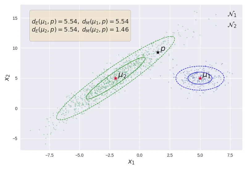
Illustration of Mahalanobis distance and Euclidean distance.

The above figure shows the effect of the underlying Gaussian distribution on the distance metric. Although the point \(\mathbf p\) is equidistant from both the points \(\boldsymbol \mu_1\) and \(\boldsymbol \mu_2\), the Mahalanobis distance \(d_M(\boldsymbol \mu_2, \mathbf p)\) is less than \(d_M(\boldsymbol \mu_1, \mathbf p)\) owing to the fact that \(\mathcal N_2\) (shown in green) has a larger variance compared to \(\mathcal N_1\) (shown in blue). As shown, \(\mathbf p\) lies within the \(2\sigma\) of \(\boldsymbol \mu_2\) compared to \(>5\sigma\) away from \(\boldsymbol \mu_1\).

Also, note that \(d_E(\boldsymbol \mu_1, \mathbf p) = d_M(\boldsymbol \mu_1, \mathbf p)\). This indicates that the euclidean distance actually assumes that the underlying data generating distribution is a standard normal distribution (i.e. unit variance across all dimensions, with no correlation). Assuming that the underlying distribution is Gaussian, the Mahalanobis distance can be seen as a generalization of the Euclidean distance from the standard Gaussian to any given covariance matrix.

Extending to GMMs

  How about a mixture of Gaussians? The Gaussian Mixture Model (GMM) is simple a weighted sum of independent Gaussian distributions. It can capture more complex distributions compared to simple Gaussian distribution without needing sophisticated computations.

Consider the GMM defined as

\[ \begin{aligned} p(\mathbf x|k) &= \frac{1}{\sqrt{(2\pi)^d |S_k|}} \exp \bigg \{ -\frac{1}{2} (\mathbf x - \boldsymbol \mu_k)^T S_k^{-1}(\mathbf x - \boldsymbol \mu_k) \bigg \} \\ p(\mathbf x) &= \sum_{k} \lambda_k p(\mathbf x|k) \end{aligned} \]

Where \(p(\mathbf x|k)\) is the \(k^{th}\) Gaussian distribution with parameters \(\boldsymbol \mu_k, S_k\) and \(\lambda_k\) is the coefficient of the \(k^{th}\) Gaussian.

To extend the idea of Mahalanobis distance to GMMs, we first need a concrete and a general idea about the distance metric - one that generalizes to any given manifold or distribution and not just a Gaussian. Such a distance is called Riemannian distance.

The local distance between two points \(\mathbf x_i\) and \(\mathbf x_j\) is determined by the space that it lies in. The data always lies on a manifold. The manifold might be of the same dimension as the ambient space itself, or may even have a lower dimension. This manifold is determined by the data-generating distribution \(q(\mathbf x)\). The data is sampled from this data distribution which defines the manifold in which the data exists^[1]. Therefore, the Riemannian distance \(d_R\) is given by the path integral between \(\mathbf x_i \to \mathbf x_j\) along the manifold, weighted by the local Riemannian metric \(G\).

\[ \begin{aligned} d_R(\mathbf x_i, \mathbf x_j) &= \int_\gamma \sqrt{(\mathbf x_i - \mathbf x_j)^TG(\mathbf x_i - \mathbf x_j)} dt && {\color{OrangeRed} \text{(Riemann Distance)}}\\ G(\mathbf x) &= \nabla_{\mathbf x}p(\mathbf x)(\nabla_{\mathbf x}p(\mathbf x))^T \end{aligned} \]

Where \(G(\mathbf x)\) is the local Riemannian metric induced by the data generating distribution \(p(\mathbf x)\). You can think of it being a generalization of the covariance matrix to arbitrary distributions. In fact, the above matrix \(G\) is called as a Fisher-Rao metric. The Fisher-Rao metric is a Riemannian metric on finite-dimensional statistical manifolds. The Riemannian metric is rather far more general.

Simplifying Riemannian Distance

The above Riemannian distance is generally intractable and the Fisher-Rao metric is also computationally expensive. There is, however, an alternate way proposed by Michael E. Tipping^[2]. Instead of the above Fisher-Rao metric, we can construct an alternate Riemannian metric for GMMs as

\[ G(\mathbf x) = \sum_{k} p(k|\mathbf x)S_k^{-1} \]

Which is simply the average of the individual inverse covariance matrices. To circumvent the intractability of equation (4), Tipping offers a tractable approximation that yields a distance metric of the same form as (2).

\[ d_{GMM}(\mathbf x_i, \mathbf x_j) = \sqrt{(\mathbf x_i - \mathbf x_j)^TG(\mathbf x)(\mathbf x_i - \mathbf x_j)} \]

Essentially we have moved the path integral inside the square-root where it is entirely captured by the local Riemannian metric \(G(\mathbf x)\). Moving from \(\mathbf x_i \to \mathbf x_j\), the Riemannian metric becomes

\[ \begin{aligned} G(\mathbf x) &= \sum_{k} p(k|\mathbf x)S_k^{-1} \\ &= \sum_{k} \frac{p(\mathbf x|k) p(k) } {p(\mathbf x)} S_k^{-1}\\ &= \frac{\sum_{k} S_k^{-1} \lambda_k \int_{\mathbf x_i}^{\mathbf x_j} p(\mathbf x|k) d\mathbf x } {\sum_{k} \lambda_k \int_{\mathbf x_i}^{\mathbf x_j} p(\mathbf x|k) d\mathbf x} && \big ( p(k) = \lambda_k \big )\\ \end{aligned} \]

Where the path integral term \(\int_{\mathbf x_i}^{\mathbf x_j} p(\mathbf x|k) d\mathbf x\) computes the density along \(\mathbf x_i \to \mathbf x_j\). If we assume that \(\mathbf x_i\) and \(\mathbf x_j\) are close to each other and that the geodesic distance can be approximated by a straight line, then

\[ \begin{aligned} \int_{\mathbf x_i}^{\mathbf x_j} p(\mathbf x|k) d\mathbf x &= \sqrt{\frac{\pi}{2a}} \exp\{-Z / 2\} \bigg [ \text{erf}{ \bigg (\frac{b + a}{\sqrt{2a}} \bigg ) - \text{erf} \bigg (\frac{b}{\sqrt{2a}} \bigg )} \bigg ] \\ \text{Where}, \quad a &= \mathbf v^T S_k^{-1} \mathbf v \\ b &= \mathbf v^T S_k^{-1}\mathbf u \\ g &= \mathbf u^T S_k^{-1}\mathbf u \\ Z &= g + b / a \\ \mathbf v &= \mathbf x_j - \mathbf x_i \\ \mathbf u &= \mathbf x_i - \boldsymbol \mu_k \end{aligned} \]

We can make some observations about the above result. First, for \(k=1\), the above equation yields the Mahalanobis distance \(d_M\) as expected. The Riemannian metric \(G(\mathbf x)\) only depends on the Gaussian components that have non-zero value along the path \(\mathbf x_i \to \mathbf x_j\), so there are no spurious influences from other component densities. Lastly, just like Mahalanobis distance the above GMM-distance is also invariant to linear transformations of the variables.

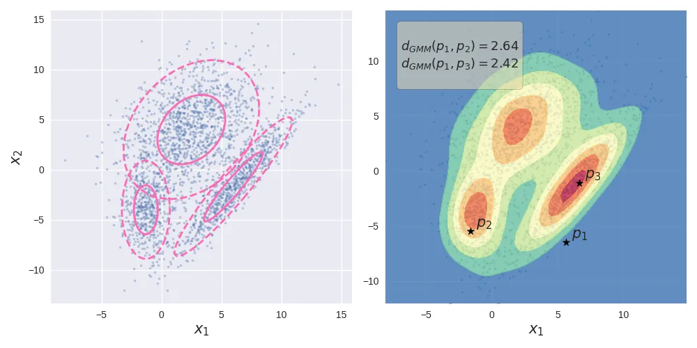
Gaussian Mixture Model. The left image shows the data generated by a mixture of 3 Gaussians. The image of the right shows the probability density along with the GMM-distances of 3 points.

import numpy as np
from scipy import special

def GMMDist(x1: np.array, x2:np.array, 
            mu: np.array, Sigma:np.array, lambdas:np.array) -> float:
    """
    Computes the Riemannian distance for Gaussian Mixture Models.
    Args:
        x1(np.array): Input point
        x2 (np.array): Input point
        mu (np.array): List of mean vectors of the GMM
        Sigma (np.array): List of Covariance matrices of the GMM
        lambdas (np.array): Coefficients of the Gaussiam mixtures

    Returns:
        float: Riemannian distance between x1 and x2 
               for the given GMM model
    """

    v = x2 - x1
    K = len(Sigma) # Number of components in the mixture
    S_inv = np.array([np.linalg.inv(Sigma[i]) for i in range(K)])

    # Path Integral Calculation
    path_int = np.zeros(K)

    def _compute_k_path_integral(k:int):
        a = v.T @ S_inv[k] @ v
        u = x1 - mu[k]
        b = v.T @ S_inv[k] @ u
        g = u.T @ S_inv[k] @ u
        # Normalization Constant
        Z = -g + (b**2 / a)

        const = np.sqrt(np.pi / (2* a))
        path_int[k] = const * np.exp(0.5 * Z)
        path_int[k] *= (special.erf((b+a)/np.sqrt(2 * a)) - 
                        special.erf(b/np.sqrt(2 * a)))

    # Compute the path integral over each component
    for k in range(K):
        _compute_k_path_integral(k)

    # Reweight the inverse covariance matrices with the 
    # path integral and the mixture coefficient
    w = lambdas * path_int
    
    eps = np.finfo(float).eps 
    G = (S_inv*w[:, None, None]).sum(0) / (w.sum() + eps)

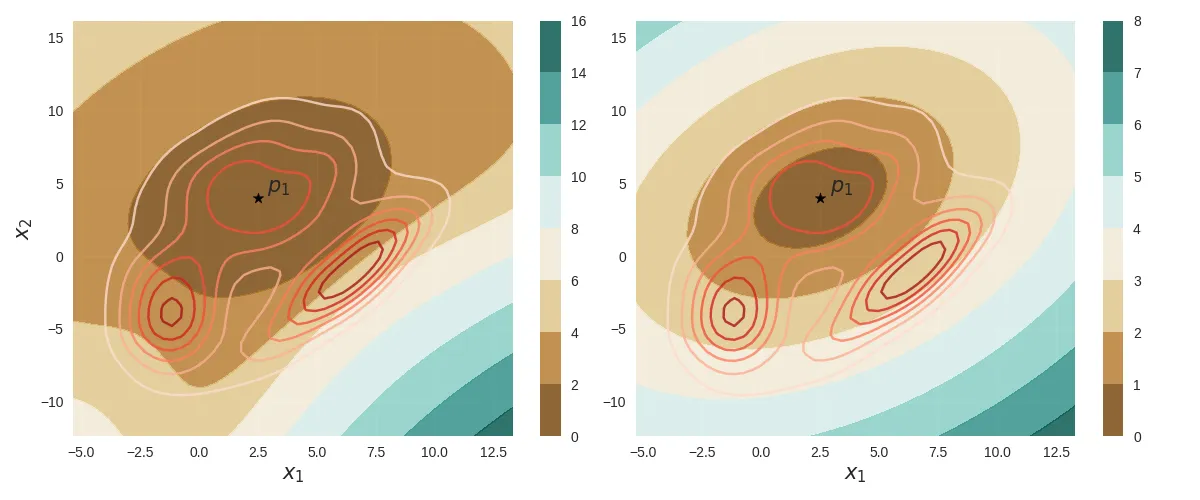
    return np.sqrt(np.dot(np.dot(v.T, G), v))

Finally, the following figure compares the contour plots of both the GMM Riemannian distance \(d_{GMM}\) (left) and the the Mahalanobis distance \(d_M\) (right) from the point \(p_1\) with the same underlying probability density (shown as red contour lines).

The clustering problem is a direct application of the above distance metrics - more specifically the class of model-based clustering techniques. Given some data samples, we fit a model (inductive bias) - say a Gaussian or a GMM, and we can use the above distance metrics to group them into clusters. Or even detect outliers.

---

[1]	As long we are dealing with data samples, it is almost always good to think of the data as samples from some data-generating distribution and that probability distribution lies on a manifold called statistical manifold. This idea has been quite fruitful in a variety of areas within ML.

[2]	Tipping, M. E. (1999). Deriving cluster analytic distance functions from Gaussian mixture models. Link.