Consider the following problem -

Given a tensor (multi-dimensional array) \(\mathbf X\) of size \(N \times L \times D\) where \(N\) is the number of samples of some numerical object of size \(L \times D\). How do you efficiently compute the sample covariance matrix of the tensor \(\mathbf X\).

I have come across the above problem more often, under different contexts, than you might assume. For instance in Machine Learning, the tensor \(\mathbf X\) can be formed accumulating \(L\) feature maps (say, from different layers of some neural network) each of dimension \(D\) from \(N\) input samples. Computing covariance can be crucial to understand how those features compare with each other across the layers. It can also be used to in feature selection. Learning to compute the sample covariance can also provide insights into computing other metrics for feature selection, finding independent features, comparing the features of two networks^[1] and so on.

Note: I will be shuttling between Numpy and PyTorch for the implementations.

Lets take a quick random tensor to work with.

import numpy as np
import torch

N, L, D = 100, 10, 5
X = 100*torch.rand(N, L, D) + 1
X_np = X.numpy()

To compute the covariance matrix of size \(L \times D \times D\), we can use Numpy's cov.

def numpy_cov(x: np.array) -> np.array:
    """
    Computes the unbiased sample covariance of the tensor x.
        S(x) = 1/(N - 1) ∑ (x - μ)(x - μ)^T
    """
    npcov = np.zeros((L, D, D))
    for i in range(L):
        X = x[:, i, :]
        npcov[i] = np.cov(X, rowvar=False, ddof=1) \
                    + 0.01 * np.eye(D).astype(np.float32) # Diagonal jitter
        # ddof = 1 for Bessel's correction
    return npcov

Unfortunately, we have to resort to manual computation in case of PyTorch as it still does not have cov function as of 1.9.0 version. Obviously we would like to have vectorized solution rather than looping over the data samples. Recall the definition of sample covariance.

\[ S(\mathbf X) = \frac{1}{N-1} \sum_{i=1}^N (\mathbf x_i - \hat{\boldsymbol \mu})(\mathbf x_i - \hat{\boldsymbol \mu})^T \]

Where \(\hat{\boldsymbol \mu}\) is the current sample mean. The main obstacle in direct vectorized computation is the subtraction of the sample mean. Computing mean and subtracting it from the elements is a sequential operation. Can this be vectorized? By this I mean a matrix \(\mathbf J\) which when multiplied by some other matrix \(\mathbf P\), subtracts the mean of that matrix across some dimension. We can construct \(\mathbf J\) as follows -

1. The sum of all elements of \(\mathbf P\) across some dimension can be computed by multiplying with a matrix of 1s.

P = torch.randn(5,5)
J = torch.ones(5,5)
assert torch.allclose(J @ P , P.sum(0).expand(5,5))
assert torch.allclose(P @ J , P.sum(1).expand(5,5).t_())

2. The sample mean can be computed if we simply divide the result by \(N\). But this can be incorporated within the matrix \(\mathbf J\).

P = torch.randn(5,5)
J = (1/5)*torch.ones(5,5)
assert torch.allclose(J @ P , P.mean(0).expand(5,5))
assert torch.allclose(P @ J , P.mean(1).expand(5,5).t_())

3. Now we can simply subtract the computed mean as P - P @ J => P(I - J) => P @ J'. This matrix is called as the centering matrix in literature and is commonly used in vectorized computation of covariances, HSIC metrics, and standardizing data. We can now directly compute our sample covariance in a vectorized form.

X = x.transpose(0, 1) # To make our life easier

J = (1.0/(N - 1))*(torch.eye(N) - (1.0/(N)*torch.ones(N,N))) # Centering matrix
gtcov = X.transpose(1,2) @ J[None, :, :] @ X # Broadcast J over dimensions of X

A slight improvement to the above gtcov computation step is to use unsqueeze() rather than None for broadcasting \(\mathbf J\) over the dimensions of \(\mathbf X\).

Note: As another slight optimization, we can add brackets to gtcov computation based on the actual values of \(L\) and \(D\). If \(L > D\), which it usually is, gtcov = (X.transpose(1,2) @ J[None, :, :]) @ X gives a small speed up.

def torch_veccov(x: torch.Tensor) -> torch.Tensor:
    X = x.transpose(0, 1) # To make our life easier
    J = (1.0/(N - 1))*(torch.eye(N) - (1.0/(N)*torch.ones(N,N))) # Centering matrix

    gtcov = (X.transpose(1,2) @ J.unsqueeze(0)) @ X # More efficient

    torch.einsum('ijj->ij', gtcov)[...] += 0.01 # Diagonal jitter
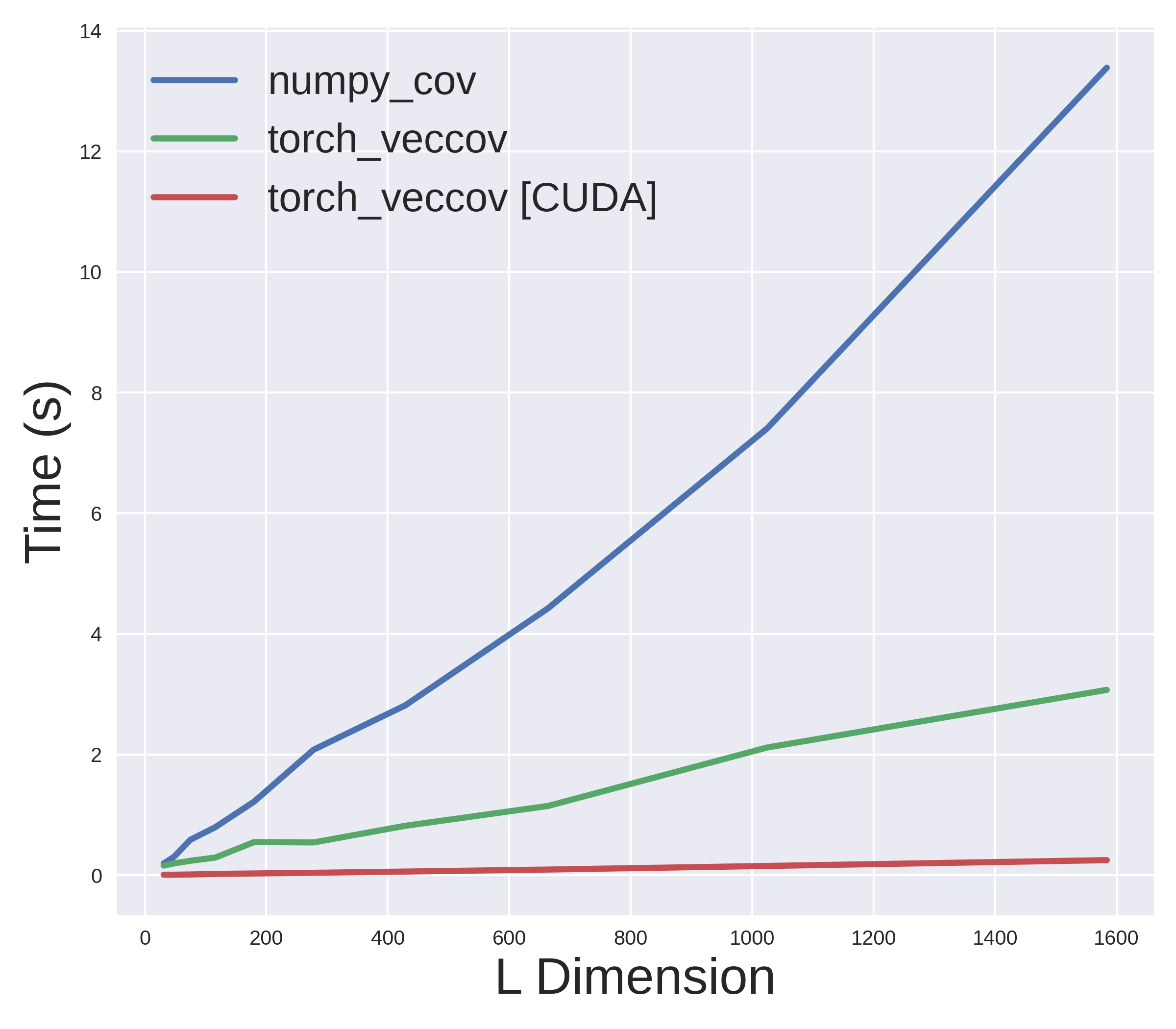
    return gtcov

Furthermore, we can also leverage PyTorch's amazing CUDA support to run the above function on the GPU without any change. Lets now compare how fast these methods actually are. The following plot shows the results for \(N = 500, D= 500\) on a machine with Intel Core i7-8750H CPU and NVIDIA RTX 2070 GPU.

But What about Streaming Data?

Granted that we can't possibly assume that we have the complete data at all times. Even if we do, it is always a good idea to process in batches for scalability and performance. So can we incorporate our vectorized solution into a streaming data framework?

From the definition of sample covariance, we have

\[ \begin{aligned} S_i &= \frac{1}{N-1} \sum_{i=1}^N (\mathbf x_i - \hat{\boldsymbol \mu})(\mathbf x_i - \hat{\boldsymbol \mu})^T \\ &= \frac{1}{N-1} \sum_{i=1}^N \mathbf x_i \mathbf x_i^T - \frac{N}{N-1}\hat{\boldsymbol \mu}\hat{\boldsymbol \mu}^T \\ \end{aligned} \]

So, we have to keep track of the sum of products of the incoming \(\mathbf x_i\) and the mean \(\hat{\boldsymbol \mu}\). We can efficiently do both the operations in-place using PyTorch's add_ and baddbmm_. The implementation is given below.

def torch_seqcov(x):
    """
    Computes the sequential unbiased sample covariance of the tensor x.
        S(x) = 1/(N - 1) ∑ xx^2 - N / (N - 1) μμ^T
    """

    mean =  torch.zeros( L, D) # feature mapsize x num features
    x2 = torch.zeros(L, D,D)

    x =  x.transpose(1,0)
    for i in range(N):
        X = x[:, i, :][ :, None, :]
        mean1.add_( X.squeeze() / (N)) # In case of minibatch, sum them

        x2.baddbmm_(X.transpose(1, 2),  X)  # x2 <- x2 + X.transpose(1, 2) @  X

    cov = (x2 / (N-1)) - ((N / (N - 1)) * mean1.unsqueeze(-1) @ mean1.unsqueeze(-2))

    torch.einsum('ijj->ij', cov)[...] += 0.01 
    return cov

With such a simple procedure, we can compute the covariance of tensors even for very large datasets.

Note: There is another formula for sequential calculation of covariance matrices that is commonly given.

\[ S_i = \frac{N - 2}{N-1} S_{i-1} + \frac{1}{N} (\mathbf x_i - \hat{\boldsymbol \mu})(\mathbf x_i - \hat{\boldsymbol \mu})^T \]

The above formula is just a few steps away from equation (2) (full derivation is shown here). However, in practice it does not work well due to the need for proper initialization and is often numerically unstable^[2].

It is quite fascinating that an intermediate step in a mathematical procedure yields numerically efficient implementation rather than the final, supposedly more beautiful, result.

---

[1]	Looking at you, Hilbert-Schmidt Independence Criterion (HSIC) 😏

[2]	Although, this has been addressed by the Welford's online algorithm.