The Back-Gradient Trick

The back-gradient trick is a method for gradient-based optimization applied to bi-level problems. A common example of such a problem is the hyperparameter optimization of neural networks. Given a neural network \(f: \mathbb R^N \to \mathbb R^M\), with parameters \(\boldsymbol \theta\) and hyperparameters \(\boldsymbol \lambda\), the problem is to find the optimal set of hyperparameters that maximizes the given objective.

\[ \begin{aligned} & \underset{\boldsymbol \lambda}{\mathop{\mathrm{argmin}} \;} L(\mathbf y, f(\mathbf x; \boldsymbol \theta^*, \boldsymbol \lambda)) && {\color{OrangeRed} \text{outer loop}}\\ & \text{s.t} \quad \boldsymbol \theta^* \in \underset{\boldsymbol \theta}{\mathop{\mathrm{argmin}} \;} L(\mathbf y, f(\mathbf x; \boldsymbol \theta, \boldsymbol \lambda)) && {\color{Teal} \text{inner loop}} \end{aligned} \]

Where \(L\) is the loss function, \(\mathbf x\) and \(\mathbf y\) are the data samples and the target respectively. In practice, the constraint optimizing the weights \(\boldsymbol \theta\) is called the inner loop, and the hyperparameter optimization the outer loop.

Usually, such problems are solved by gradient-free model-specific methods like random sampling, grid sampling, and evolutionary algorithms. Furthermore, the above is just one instance of a bi-level optimization. Another interesting example is the gradient-based adversarial attack, in which the attacker designs a surrogate model by training on a set of "poisonous" data points such that the model misclassifies new poisonous data, favourable to the attacker. The poisonous data generation is the outer-loop, while the model optimization is the inner-loop.

To understand why bi-level optimization is hard, note that the outer loop requires that the inner loop is run till optimum and that the entire trace i.e. the intermediate values of the inner loop from the initial parameters to the final optimum parameters are available. These are practically unreasonable requirements for any model with more than a dozen parameters. This is the main reason why hyperparameter optimization is mostly done by gradient-free methods - they don't require the entire trace and the inner loop needn't be differentiable.

Gradient-based and search0based hyper-parameter optimization.

The Core Problem

Consider the usual gradient-descent update for optimizing the network parameters \(\boldsymbol \theta\).

\[ \begin{aligned} \boldsymbol \theta_{t+1} &= \boldsymbol \theta_t - \alpha \nabla \boldsymbol \theta_t \qquad t = 1,2,..., T \end{aligned} \]

Where \(\nabla \boldsymbol \theta = \nabla_{\boldsymbol \theta} f(\mathbf x_{t}; \boldsymbol \theta_t, \boldsymbol \lambda)\) and \(\alpha\) is the learning rate. The convergence guarantees of SGD imply that the above procedure yields the near-optimum \(\boldsymbol \theta_T \approxeq \boldsymbol \theta^*\) after a certain number of updates, irrespective of the initial \(\boldsymbol \theta_1\), even with the same hyper-parameters \(\boldsymbol \lambda\).

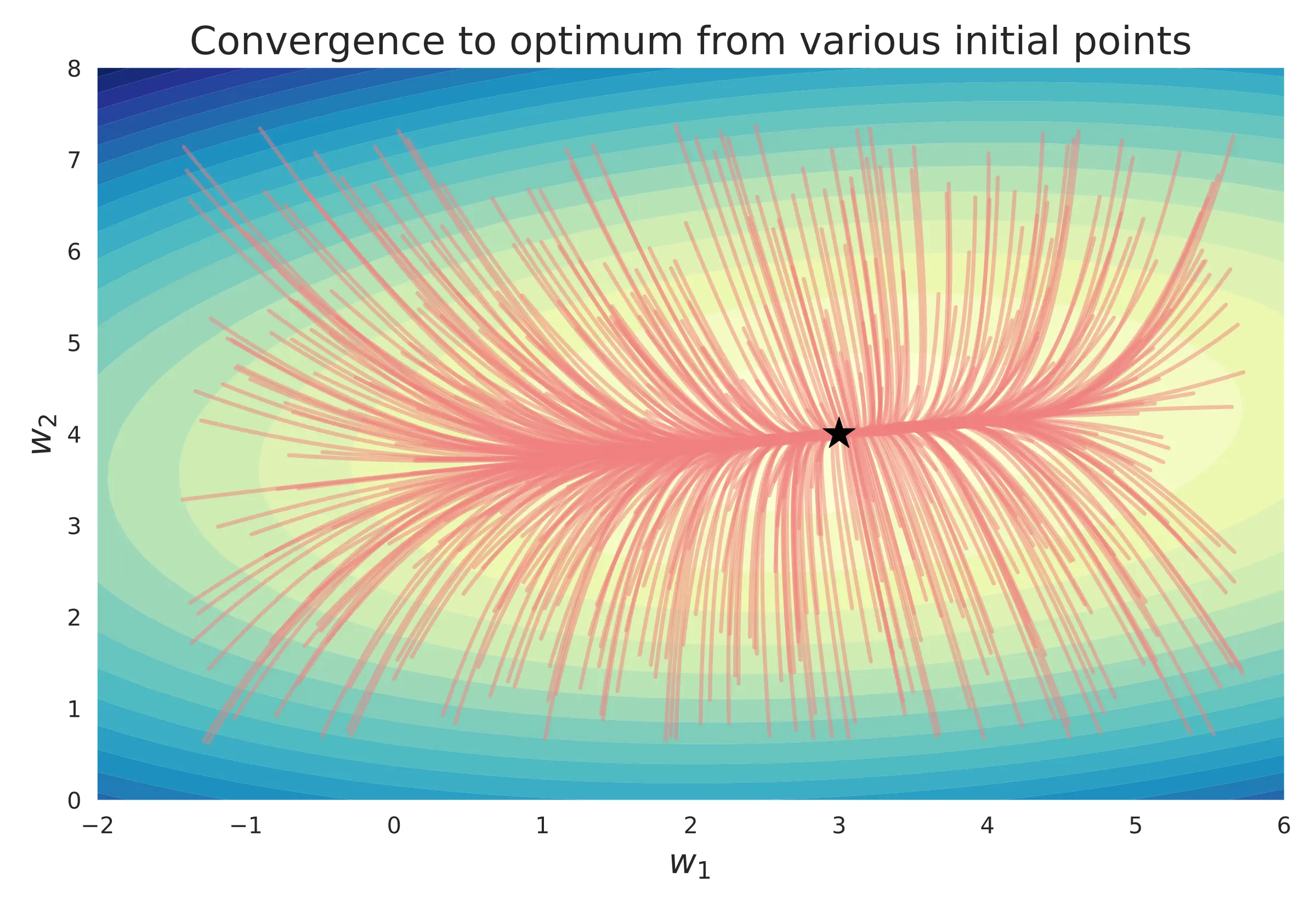
Convergence of SGD to optimum from different initial points.

From the above graph, it is clear that there is no, or rather shouldn't be, one-to-one mapping between the initial points and the optimum. A good optimizer should converge to the optimum from any initial point. However, back-tracing requires that the mapping be one-to-one i.e. reversible. How do we resolve this apparent paradox? It is resolved from the observation that each step of the gradient descent update is bijective and can be exactly inverted. The entire trace is a series of small bijective mappings and the convergence to the optimum hinges on the local gradient. If we can retrieve the local gradient exactly, we can reverse the entire trace!

Note: The above contours represent the loss landscape and not the \(\lambda-\theta\) space. Even when the loss landscape has one (simple) global minimum, as shown above, the \(\lambda-\theta\) space can have multiple optima.

Mathematically, unrolled version of equation (2) can be constructed as function \(h : \mathbb R^{|\boldsymbol \theta|} \times \mathbb R^{|\boldsymbol \lambda|} \to \mathbb R^{|\boldsymbol \theta|}\) which takes in the inputs \(\boldsymbol \lambda\) and the initial parameters \(\boldsymbol \theta_1\) and outputs the trained parameters \(\boldsymbol \theta_T\).

\[ h(\boldsymbol \lambda, \boldsymbol \theta_1) = \boldsymbol \theta_T \]

The function \(h\) represents the trajectory of points \(\boldsymbol \theta_1 \to \boldsymbol \theta_T\), and itself represents a (massive) computational graph. The task now is to address the irreversibility of the above function to obtain the hyperparameter gradient \(\nabla \boldsymbol \lambda\).

Back-Gradient Trick

Observe that the equations of the gradient descent, like equation (2), are reversible. One can easily obtain \(\boldsymbol \theta_t\) from \(\boldsymbol \theta_{t+1}\) given \(\nabla \boldsymbol \theta_t\). Therefore, the naïve method is to store every intermediate weight gradients \(\nabla \boldsymbol \theta_1, \nabla \boldsymbol \theta_2, \ldots, \nabla \boldsymbol \theta_T\) for traversing back across \(h\) ^[1].

However, this method is quite memory intensive and becomes impractical even for medium-sized problems \((\dim(\theta) \geq 10^2)\) as this requires storing weights at every optimization step. The memory complexity would be \(\mathcal O(L|\theta|)\) where the number of iterations \(L\) can be in 1000s. Furthermore, if the gradient descent algorithm becomes a bit more sophisticated like heavy-ball momentum, Nesterov's momentum, and RMSprop, then all their intermediate values also need to be stored.

An alternative method is the back-gradient method^[2] where each step of the gradient descent is reversed, instead of the whole trace \(h\). In each step, the gradient is recomputed, rather than stored.

\[ \begin{aligned} \nabla \boldsymbol \theta_t &= \nabla_{\boldsymbol \theta} f(\mathbf x; \boldsymbol \theta_t, \boldsymbol \lambda) \\ \boldsymbol \theta_{t-1} &= \boldsymbol \theta_t + \alpha \nabla \boldsymbol \theta_t \qquad t = T, T-1, T-2, \ldots, 1 \end{aligned} \]

with \(\nabla \boldsymbol \theta_T = \nabla_{\boldsymbol \theta} f(\mathbf x; \boldsymbol \theta_T, \boldsymbol \lambda)\) as initial value. This method is indeed scalable, without needing to store every intermediate value, even for more sophisticated algorithms.

The above computation, however, is highly sensitive. Recall that near the optimum \(\boldsymbol \theta^*\), multiple trajectories from different initial points converge together. As such, it is practically impossible to differentiate one trajectory from another. Even at high precision, the tiniest numerical difference would cause the back trajectory to be vastly different from the original trajectory. This phenomenon occurs at any region where multiple trajectories converge like attractors, plateaus, and saddle points ^[3].

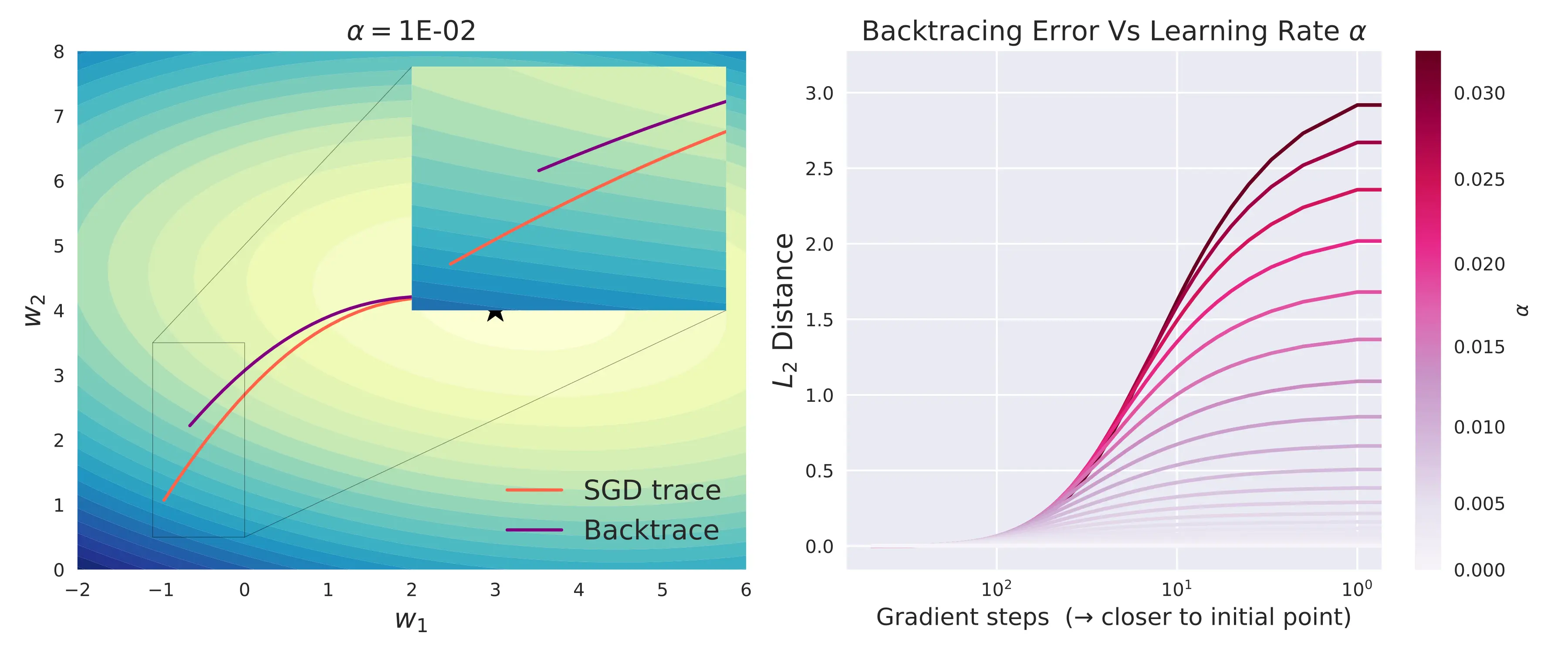
The above figure illustrates that even for a simple 2D linear model, with just 500 gradient steps at 64-bit precision, there is a significant difference in the forward and backward traces. For more complex neural networks with hundreds of thousands of weights and thousands of gradient steps across a difficult loss landscape, this method would fail miserably.

Notice that the error tends to zero as \(\alpha \to 0\). But \(\alpha > 0\) is necessary for convergence. The fundamental issue here is the lossy nature of floating-point multiplication. Although multiplication is ideally a reversible operation, floating point multiplication often loses bits (information) due to rounding or cancellation. A tiny deviation in the result of multiplication causes the gradient evaluated to be significantly different. The problem has, now, transformed into a numerical one.

Reversible Floating-Point Operations

To make floating point multiplication reversible, we convert weights to 64-bit integers and the \(\alpha\), \(\beta\) factors as a ratio of integers as they are rational in practice. For example, if the weight were a 64-bit integer, say 4365, and the floating-point value to be multiplied is 0.875 (represented as 7/8), then the updated weight is (4365 // 8) * 7 = 3815, where// is integer division. There is a reminder of 5 that needs to be carried over for exact reversibility i.e to get 4365 from 3815 when divided by 7/8. This can be stored and tracked in some buffer b, which is another 64-bit integer. In the above example, the reminder can be safely added to the result to get 3820 and our final result.

def rational_mul(w, n, d):
    """
    Rational multiplication that 
    handles reminders
    """
    b = w % d  # buffer
    w = w // d
    w = w * n
    w = w + b
    return w

def exact_mul(w, n, d):
    """
    Exact multiplication
    """
    return rational_mul(w, n, d)

def exact_unmul(w, n, d): 
    """
    Exact inverse of multiplication
    """
    return rational_mul(w, d, n) # notice order of arguments

w = 4365
w = exact_mul(w, 7, 8)   # w = 3820
w = exact_unmul(w, 7, 8) # w = 4365

The above method works as long as there are no underflows or overflows. Buffers can also be used to track overflows and underflows. Furthermore, how do we convert floats to int and back? One way is to multiply by some big integer, sufficient to fit into the 64-bit integer like \(2^{52}\) and the original value can be retrieved using division. This complete implementation including all these modifications for JAX arrays is given below ^[4].

# Based on https://github.com/bkj/mammoth
_double_cast = lambda x: x.astype(jnp.float64)

class ExactArray:
    # 52 = Significand precision in 64-bit float
    RADIX_SCALE = int(2 ** 52) 

    def __init__(self, val: jnp.array):
        self._cast = _double_cast

        self.intrep = self.float_to_intrep(val)
        
        # Auxiliary variable to store and track reminders
        self.aux = jnp.zeros_like(val).astype(jnp.int64) 

        # List to store overflowed auxiliary variables
        self.aux_buffer = []
        self.aux_pushed_at = [0]
        
        self.counter = 0
    
    def _buffer(self, r, n, d) -> int:
        assert jax.lax.le(d, 2 ** 16).all(), 'ETensor_jax._buffer: M > 2 ** 16'
        self.aux *= d 
        self.aux += r
        
        rem = self.aux % n
        self.aux = self.aux // n
        
        return rem
    
    def add(self, a):
        self.intrep += self.float_to_intrep(a)
        return self
    
    def sub(self, a):
        self.add(-a)
        return self
    
    def rational_mul(self, n, d) -> None:
        r = self.intrep % d
        rem = self._buffer(r, n, d)
        
        self.intrep -= self.intrep % d 
        self.intrep = self.intrep // d
        self.intrep *= n
        self.intrep += rem
    
    def float_to_rational(self, a) -> Tuple:
        assert jax.lax.gt(a, 0.0).all(), "0.0 is not rational!"
        d = (2 ** 16 / jnp.floor(a + 1)).astype(jnp.int64)
        n = jnp.floor(a * self._cast(d) + 1).astype(jnp.int64)
        return (n, d)
    
    def float_to_intrep(self, x) -> jnp.array:
        if isinstance(x, float):
            x = jnp.array([x])
        intrep = (x * self.RADIX_SCALE).astype(jnp.int64)
        return intrep

    def mul(self, a: float):
        n, d = self.float_to_rational(a)
        self.rational_mul(n, d)
        
        self.counter += 1
        # If true, then could overflow on next iteration
        if self.aux.max() > 2 ** (63 - 16):
            self.aux_buffer.append(self.aux)
            self.aux = jnp.zeros_like(self.aux)# !! Fastest way?
            self.aux_pushed_at.append(self.counter)
        
        return self
    
    def unmul(self, a: float): # Reversing mul operation
        # Check for overflows/underflows at current operation
        if self.counter == self.aux_pushed_at[-1]:
            assert (self.aux == 0).all()
            self.aux = self.aux_buffer.pop()
            _ = self.aux_pushed_at.pop()
        
        self.counter -= 1
        
        n, d = self.float_to_rational(a)
        self.rational_mul(d, n) 
        return self
    
    @property
    def val(self):
        return self._cast(self.intrep) / self.RADIX_SCALE

Now that we have the above data structure ExactArray that can perform multiplication without loss in information, we can use it for the weights and other intermediate variables of the optimizer for exact reversibility.

import jax
from typing import Tuple

"""
Prerequisites:
model, loss_fun, x (data)
"""

grad_loss_fun = jax.grad(loss_fun, argnums=0)

def sgd_m(state:Tuple, 
          alpha:float, 
          gamma:float,
          **kwargs) -> Tuple:
    """
    SGD +  Nestorov Momentum that can be
    backtraced.

    Update equations :
    v = gamma * v + w_grad
    w = w - alpha * v

    Args:
    state  = Tuple containing 
            (weights:  ExactArray,
             velocity: ExactArray)
    alpha  = learning rate
    gamma  = mass for momentum

    Usage:
    for i in range(MAX_ITER):
        state = sgd_m(state, alpha = 1e-2, gamma=0.8)
    """
    W, V = state
    w_grad = grad_loss_fun(W.val, x)
    V.mul(gamma).sub(w_grad).add(beta).mul(alpha)

    W.sub(V.val)
    return (W, V)

def backtrace_sgd_m(state:Tuple, 
                    alpha:float, 
                    gamma:float, 
                    **kwargs) -> Tuple:
    """
    Backtraces SGD + Nestorov Momentum exactly.

    Args:
    state  = Tuple containing 
            (weights:  ExactArray,
             velocity: ExactArray)
    alpha  = learning rate
    gamma  = mass for momentum

    Usage:
    # Get the last state from sgd_m
    for i in range(MAX_ITER - 1, -1, -1):
        state = backtrace_sgd_m(state, alpha = 1e-2, gamma=0.8)
    """
    W, V = state
    W.add(V.val)
    w_grad = grad_loss_fun(W.val, x)
    V.unmul(alpha).sub(beta).add(w_grad).unmul(gamma)

    return (W, V)

The above figure illustrates the exact reversibility of some simple gradient descent algorithms (for discussion about vanilla SGD, see ^[5]) with hyper-parameters \(\alpha\) and \(\gamma\). Compared to storing the entire weight (and/or corresponding gradients) at each step, we only store the final weight (along with any intermediate parameter like velocity) for reversing the entire trace.

The above technique can be extended to the other gradient descent algorithms like RMSProp and Adam, but they require careful implementation of reversible exponents (square and square root)^[6]. Nonetheless, this simple reversibility leads to gradient-based hyperparameter optimization and meta-learning techniques.

Gradients from Reversible SGD

Back to the back-gradient trick. To get the gradients we can construct the massive computational graph from the entire trace and then backpropagate. This can again be memory and time intensive to be scalable even for medium-sized models. Therefore, we can once again resort to amortizing across each step and compute the back-gradients during each reverse SGD step. In addition to being scalable, this also provides us with fine-grained control over when and how to backpropagate the hyperparameter gradients. This technique is sometimes called as online hypergradients in literature.

Consider the above SGD with Nestorov Momentum algorithm. For our example, the learning rate \(\alpha\) and the momentum mass \(\gamma\) can be considered as the hyper-parameters. We are interested in the gradients of the mode \(f\) at the final weights \(\boldsymbol \theta_T\) with respect to the hyperparameters \(\alpha\) and \(\gamma\) - represented as \(\nabla \alpha\) and \(\nabla \gamma\) respectively. The back-gradient SGD (BG-SGD) computes the hyperparameter gradients as follows -

\[ \begin{aligned} \text{SGD} & &&\text{BG-SGD}\\ \mathbf v_{t+1} &= \gamma \mathbf v_{t} &&\nabla\alpha &&= d \boldsymbol \theta^T \mathbf v_{t+1} \\ \mathbf v_{t+1} &= \mathbf v_{t+1} - (1 - \gamma) \nabla \boldsymbol \theta_t &&\boldsymbol \theta_{t} &&= \boldsymbol \theta_{t+1} - \alpha \mathbf v_{t+1} &&{\color{Teal}\text{Reverse weight update}}\\ \boldsymbol \theta_{t+1} &= \boldsymbol \theta_{t} + \alpha \mathbf v_{t+1} &&\mathbf v_{t} &&= [ \mathbf v_{t+1} + (1 - \gamma) \nabla \boldsymbol \theta_t]/\gamma &&{\color{Teal}\text{Reverse velocity update}} \\ & &&\nabla\mathbf v_{t} &&= \nabla \mathbf v_{t + 1} + \alpha d \boldsymbol \theta\\ & &&\nabla\gamma &&= \nabla \mathbf v_{t}^T (\mathbf v_{t+1} + \nabla \boldsymbol \theta_t) \\ & &&d\boldsymbol \theta && = d\boldsymbol \theta - (1 - \gamma)\nabla \mathbf v_{t} \nabla^2 \boldsymbol \theta_{t}\\ & &&\nabla\mathbf v_{t} &&= \gamma \nabla \mathbf v_{t}\\ \end{aligned} \]

The above algorithm yields the required gradients \(\nabla \alpha\) and \(\nabla \gamma\) with respect to the learned model \(f(\mathbf x; \boldsymbol \theta_T)\). The hyper-parameters can themselves be updated based on their gradients to improve the dynamics of the inner gradient descent towards a better optimum. This is often called the meta gradient descent or hyper-gradient descent.

Note: We initialize \(d\boldsymbol \theta\) with the gradient of the learned weights after SGD - \(\nabla_{\boldsymbol \theta}(f(\mathbf x; \boldsymbol \theta_T))\). This \(d\boldsymbol \theta\) represents the gradients of the final model with respect to the current weights and at the end of the back-gradient iterations will represent the gradients with respect to the initial weights \(\boldsymbol \theta_1\). This notation is employed to avoid confusion between the actual gradients at each step \(\nabla \boldsymbol \theta_t\).

Conclusion

In summary, the reversibility of the gradient-descent update leads to an innate problem in floating-point math, fixing which leads to an elegant meta gradient-descent method for optimizing the hyper-parameters. The back-gradients / hyper-gradients can be computed in \(\mathcal O(|\theta|)\) memory and \(\mathcal O(L)\) time where \(L\) is the number of inner gradient-descent steps. Based on this trick, meta-learning has indeed become more practical and has advanced tremendously in the past few years.

[1]	This observation was first made by Justin Domke in his 2012 paper.

[2]	The term back-gradient is relatively new. There have been many names used in literature like reversible learning, back optimization, and hypergradients.

[3]

From an information theoretic perspective, optimization always moves from a high-entropy initial state to a low-entropy (ideally zero-entropy) optimum. Attractors, saddle points, and plateaus are low entropy states that also cause multiple trajectories to converge towards them, besides the optimum. Once multiple trajectories converge, then they cannot be uniquely traced back.

[4]	A slightly more memory-efficient algorithm is given in Maclaurin et. al. Algorithm 3 and the code follows the same.

[5] Why isn't vanilla SGD exactly reversible? From the figure, SGD + momentum and Nestorov momentum are both exactly reversible. This is because the \(\gamma\) (akin to the mass) acts as the anchor for reversibility. In the code for momentum-based methods, both the weights and the velocity parameters are stored as ExactArrayi.e more information per step is stored compared to vanilla SGD. For exact reversibility of vanilla SGD, we have no other option but to store the entire gradient which is infeasible as discussed previously.

[6]	See Baydin et. al.'s 2018 paper for a more practical solution to this problem.